Keywords: Computer Vision, OpenCV, Python, Too much free time
Orignially posed here on Medium on March 30, 2020.
The Motivation
I have spent most of the past month indoors. First few days were on WFH amid social distancing measures in Tokyo. Then travelled back to Bangalore. Thereafter spent 14 days on home quarantine as recommended by the immigration authorities. And co-incidentally the 21 day nationwide lockdown in India started on my last day of home quarantine. This seems to be a never ending cycle of isolation and the same story is replicated across my social circle and the world in general.
In the midst of all this crisis there are a bunch of funny and sarcastic memes being forwarded on activities people are doing to get over their boredom. One that particularly piqued my interest was this one:

Here’s why. Many years ago during my time as a Research Fellow at IIT Kharagpur, I used to conduct the laboratory course for Digital Image Processing for a few semesters. And among my standard list of weekly assignments was one to write a computer vision algorithm to count the number of rice grains in this image:

So when a good friend of mine, Mithun Dhali, sent me a pic of some lentils on a piece of paper (evidently inspired by the above forward) asking me to help him to count the number of grains, it brought back nostalgic memories. So I scourged my old hard drives to look for codes written long back as reference solutions to the above problem. Took some time to locate them. The old codes were written in C and used now outdated OpenCV 1.x APIs. I no longer have the older library versions installed in my current PC and since Python is all the rage now, I decided to port the logic to Python 3 code using the latest OpenCV APIs.
In this post, I will demo the very simple steps to implement the above solution, explaining some of the algorithm choices that were made, some alternatives and limitations of the solution presented here. Note that this is a purely Computer Vision algorithm solution in a time where Deep Learning seems to be the universal hammer for nails of all kinds so do bear with me this transgression.
Simplifying the problem
Pixels in an image can take a large range of values, even the ones representing same or similar objects. This poses particular hurdles to solving image understanding tasks using classical computer vision algorithm steps. In our input grayscale image the values represent various shades of grey ranging from 0 to 255 of the 8-bit image representation. The boundaries of values separating one type of object from another are not always clear and may have significant range overlap due to lighting conditions during the image acquisition. The standard approach is to reduce the values to a handful of distinct values, each representing meaningful objects. This is known as segmentation. In this case, we only have two types of regions within the image. One is the group of pixels belonging to the rice grains, and the other belonging to the background void. This is a very common special case known as Binary Segmentation i.e., transform the input grayscale image into a pure black and white form. Pure white depicting the pixels of the rice grains and pure black depicting the universal background. Once this is done, the problem boils down to merely counting the number of distinct pure white objects in the image. There are a number of differing ways to achieve the above.
Binary Thresholding with fixed threshold
thresh, output_binthresh = cv.threshold(input_rice, 127, 255, cv.THRESH_BINARY)
print("Fixed threshold", thresh)
cv.imshow("Binary Threshold (fixed)", output_binthresh)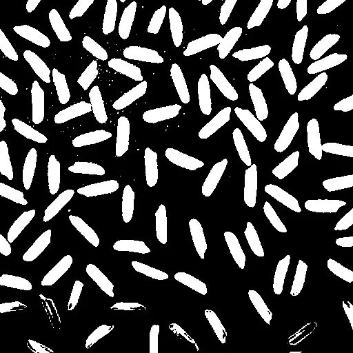
As you may have inferred, this assumes that perhaps there exists a particular value such that all rice grain pixels are brighter than that, and all background pixels are darker. For simplicity we consider that to be 127 in this case (middle of the 0–255 range). But looking at the output we do realize that quite a few background pixels have been marked white, and many of the rice grain pixels have been marked black. Now, the question is do we have to come up with a suitable threshold value by trial and error or is there a more structured way to do so ?
Binary Thresholding with Otsu’s method
Nobuyuki Otsu’s threshold selection method, more widely known as Otsu’s Method , statistically computes a suitable threshold by maximizing inter-class variance. We can use the same to achieve a better quality binary segmentation result.
thresh, output_otsuthresh = cv.threshold(input_rice, 0, 255, cv.THRESH_BINARY | cv.THRESH_OTSU)
print("Otsu threshold", thresh)
cv.imshow("Binary Threshold (otsu)", output_otsuthresh)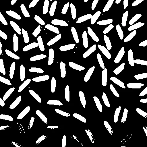
The above results are definitely cleaner than before but still not good enough. Can we do better ? The answer is YES. If we go back and observe the original input image, we can see that the entire image is not uniformly illuminated. The center region is certainly brightest. It grows darker towards the bottom and to some extent towards the top and the corners as well. This is a common scenario due to point sources of light. Therefore one single threshold over the entire image is perhaps not the best way to go about solving the binary segmentation problem.
Local Adaptive Thresholding
The solution to varying illumination is the need to determine different thresholds suitable only for limited parts of the image. What local adaptive threshold does is find a statistically suitable threshold for each pixel, depending on the distribution of pixel shades within a limited rectangular region surrounding the pixel. This negates the illumination gradient.
output_adapthresh = cv.adaptiveThreshold (input_rice, 255.0, cv.ADAPTIVE_THRESH_MEAN_C, cv.THRESH_BINARY, 51, -20.0)
cv.imshow("Adaptive Thresholding", output_adapthresh)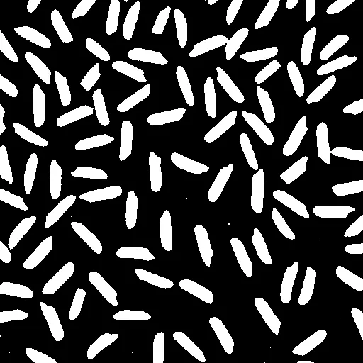
The size of the rectangular region is a tunable parameter. There is a bit of intuitive process to get it right. We chose the region size to be 51X51 pixels around each pixel, which is approx 10% of the image dimension of 512X512. Which seems to work well with the slow illumination changes as in our input sample. For rapid changing illumination a smaller region would be warranted.
Post-processing
Even with the local adaptive thresholding, that seems to perform the binary segmentation quite well, we still have minor issues leftover in the output. There are random specks of bright pixels where there is supposed to be background. Also some of the grain objects are conjoined, which may throw off the counting results. We need to clean up the segmented image to make it more amenable for accurate counting.
Morphological Erosion
Erosion is a geometric transformation to reduce aka erode the foreground shapes. We erode the image with a 5 pixel rectangular operator. This helps in removing the outlying specks. Also to separate out conjoined grain objects.
kernel = np.ones((5,5),np.uint8)
output_erosion = cv.erode(output_adapthresh, kernel)
cv.imshow(“Morphological Erosion”, output_erosion)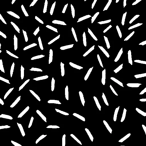
The resultant output is now fully ready for our counting algorithm.
Counting the grains
As I mentioned earlier, with proper simplification and post-processing the seemingly complex problem has been reduced to just counting the number of distinct pure white objects. I shall present two alternatives to do the same.
Connected Components
label_image = output_erosion.copy()
label_count = 0
rows, cols = label_image.shape
for j in range(rows):
for i in range(cols):
pixel = label_image[j, i]
if 255 == pixel:
label_count += 1
cv.floodFill(label_image, None, (i, j), label_count)
print("Number of foreground objects", label_count)
cv.imshow("Connected Components", label_image)
The above logic starts with systematically looking for white pixels, assigning them a unique label id (1 to 254) and the same label to all adjoining white pixels recursively till the whole distinct object is covered and labeled. Then moves on to look for the next available white pixel (255) and repeats the process till the entire image has been processed. Number of unique labels assigned is the same as distinct foreground objects i.e., grains of rice.
Contours
_, contours, _ = cv.findContours(output_erosion, cv.RETR_EXTERNAL, cv.CHAIN_APPROX_SIMPLE)
output_contour = cv.cvtColor(input_rice, cv.COLOR_GRAY2BGR)
cv.drawContours(output_contour, contours, -1, (0, 0, 255), 2)
print(“Number of detected contours”, len(contours))
cv.imshow(“Contours”, output_contour)
The contour detection logic works by finding foreground / background boundary pixels and then doing border following logic to encode the external contour shape in the form of chain codes. This is performed until the borders of all foreground objects are covered. The number of unique external contours detected is the same as the number of grains of rice.
The above algorithm does its job on the given input image but still requires manual tuning of some parameters. The same solution may not generalize enough to different inputs or under different illumination conditions. Also this will fail miserably if the density of the grains is higher in the images i.e., most grains are adjacent or occluded from one another.
The full source code can be found here https://github.com/sumandeepb/OpenCVPython
What next ?
Machine learning / deep learning based solutions may help develop a more generic solution. May even be able to handle cases of high density of grains. With more free time at hand perhaps I shall explore this further.